Jack Hales Prime Number Research Journal - 2024

Jack Hales

Dataology

me@jackhales.com

Articles Background & Experience

← Back

Jack Hales Prime Number Research Journal - 2024

A brief overview of the renewed research I've been doing on prime numbers in 2024.

By Jack Hales | 23 October 2024

23rd of October, 2024

I've taken a renewed interest in this prime number research project for a perplexity of reasons. I read and re-read a lot of Nassim Taleb, and a few of his paraphrased points have been of great influence. Specifically:

Black Swan, the middle of Chapter 11, discussing the 3-body problem: Forecasting accrues tiny compounding errors, leading to large deviations.

This leads into chaos theory, the work of Pointcarre, chaos theory and topology.

Taleb has also discussed that tinkering gives him a higher-IQ than planning to solve problems.

Finding bird poop: Researchers looking into the universe picked up hums of old radiation from the birth of the universe. They assumed it was bird poop from radar dishes, instead they were shocked with their accidental discovery.

This all comes to provide me with accidental validation that the prime number generator I am working on, and the way I was going about it, was not so bad at all. Further, it might lead to some more tools for other practitioners on handling chaos and tinkering.

To recap what I am experimenting with: Denoting an equation which predicts the next prime number.

Chaos theory, prediction application: This is a unique application where the chaos of sequential prime numbers is very volatile and maddening, but the accuracy of the sample data, and ability to generate it - is logical and functional.

Confirmation carefulness: In my previous word, confirmation was the killer. You could have a very well-fit equation at primes 1-1,000,000, and then lose it all in the next million sequential primes.

Manufactured tinkering: I am not that smart with mathematics besides the basics, so I wrote a brute force equation builder. I then created a "fitness" algorithm to rank them. This provided me with very telling equations.

P=NP: Although there is no direct link to Nth-prime, and NP complexity - there is a growing amount of computational complexity involved in finding new primes. It's also crossed my mind that these "secondary equation problems" could exist, where algorithmic problems can be solved mathematically. I have no backup for this idea!

Now that I've preambled, I am going to update this with my findings as I find them - like a journal - to assist in the valuable art of seeing events as they occur.

Creating Equations

Creating equations is an important piece of the puzzle. My first algorithm was very inefficient, and could take hours to find valuable equations by brute-forcing. My aim is to play around with building a quicker algorithm generator by understanding the form of equations deeper.

I'm also concerned that there might be logical functions that are needed that do not exist in existing mathematics which are required to express the logical pattern of primes. I cannot determine this, but if needed, I will be able to bake in custom functions into this interpreter.

This is where I left off in April last year, and I did have an interesting idea - encoding equations into integer or float matrixes, so generating could done much quicker.
The messy initial approach to generating equations, which I did in my first approach in Jan 2022, is to load in an array of possible equation parts, and generate N parts to try to successfully get an equation. Test it. If it passes, it can be used. This leads to some valid equations, but most aren't.
I'm going to have a go at building an array-based interpreter which can then construct into an expression. I am skeptical, but it might yield some better and more efficient analysis.

The above are 3 approaches to creating equations.

Creating Equations - Numeric

The first dot-point was never integrated, but I believe it is a good quickly approach. The aim is to embed the discussed expression tokens (cos, sin, (, ), etc) into a matrix. One difficulty I had with this was the embedding of floats into an equation, which I think can be solved with types. Python distinguishes between integers and floats, and we can distinguish 1.00 from 1. This way, we can leave ints for expression tokens, and floats for equation float-representations.

My first successfull (messy) implementation walked through an algorithm like:

Generate an equation length from 1-100.
Make a strand (input: length): this is a series of letters (a, s, c, g) which correspond to attachment, substitutable, constant or glue.
Make an equation by supplementing the letters for their possible values (glue = +-*/, etc).
Check the equation with a sample response to see if it's valid.

This worked well, and one assumption I am realising now is that it always started with an "attachment" to start. This was X, PI or E.

Upon implementing a very basic version to get started, raw compute suffices to build some successful equations. See the code here.

I will review this component in the future, once I have a working end-to-end fitter.

Fitting to primes

To fit the values, I have created a separate function which takes in the results of the expression, as well as the primes it is to be tested against. I'm using a cumulative absolute difference, to test against the best values. I've written this out, and now I'm going to the shops and will leave this running during that time to see what it can produce. This is the most inefficient version of what I am attempting to create using the new version, to test the approach. See here.

Properties

Properties are important, as they define what we're looking for in an equation. A straightforward one for prime numbers is:

N+1 prime number > N prime number - every prime is larger than the last.

This leads to an optimisation in the result checker, which would normally have to check over N primes we're testing against.

Reminder: The best we've got from attempt 1 and 2

The best equation I was able to fit was:

x*log(x,y) (y=7 to start, x steps by 2) - tested below further

Also:

e^cos(x) + e*x

These are interesting prime-fitting equations.

24th of October, 2024

It's clear the new modified numeric equation builder is slow. We know from the previous iteration that the above equations can exist. They would be represented as an array as such:

[
   3.00, # 3.00 float
   2, # *
   14 # log(x, y)
]

Conditions:

A randint of 3 (1% chance)
y=7 (we have a range that steps from -10 to 10 for y values)

Creates:

x*log(x,y)

When inputting this manually, we get a quite bad fitness level when we're stepping x=1,2,3, ...

In fact, y=7 is meant to be the best fitness of this equation. But we do not see that at all.

At a x step of 1, we see the best fitness is at y=3. The fitness being 1,185,775 (absolute cumulative difference to the first 1,229 primes).

What I recall from the previous project, is that there is a weird difference when we step by x=2. When we apply it here, we get what we were seeing in the past. At x=2,4,6,8,10,..., we get the best fitness at y=7, and a cumulative absolute difference of 65,995.

When we narrow down from 6-8, stepping by 0.001, we get the following fitness plot:

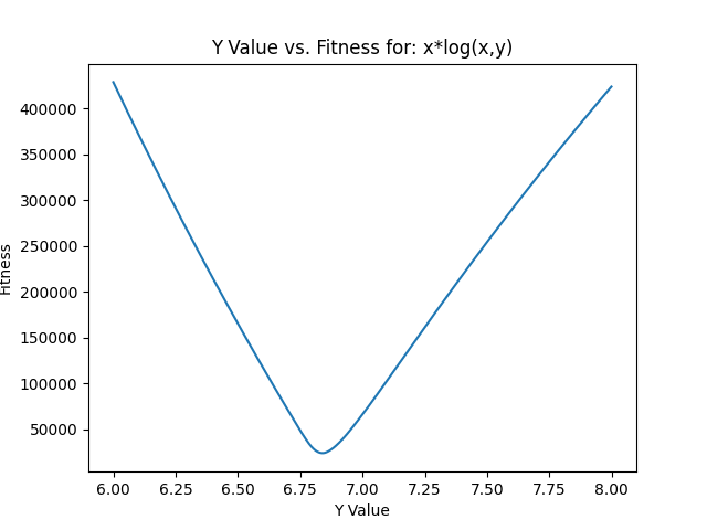
The minimum in the test is y=6.84, at a fitness of 23,710.

For your interest, here is a figure of the equation alongside the prime numbers:

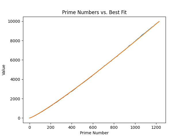
It's strikingly well-fit at this size.

And, as I am sure you are wondering, here is the difference between these - to get a slightly closer look into one of prime numbers radically beautiful visualisations:

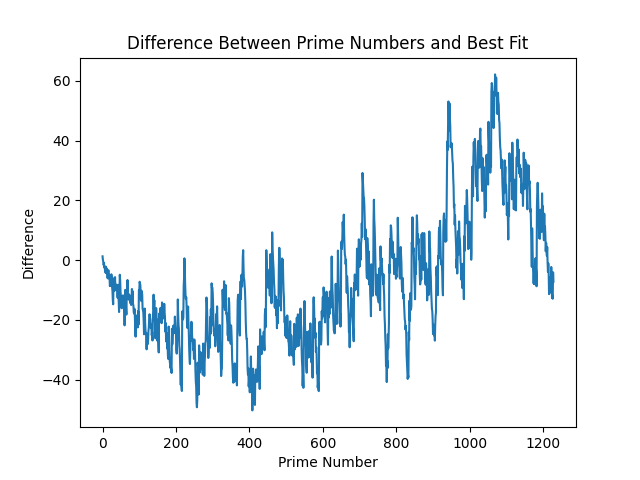
Difference in prediction and primes of x*log(x,y)

Technically, the above is all of our model errors. It becomes quickly clear why this problem has complexity baked into it - to somehow quantify this complexity into an equation. This relates back to the discussion on chaos theory (which I have studdied nothing on), and is where this article starts to touch area I've not been at before. The above are errors that accrue over time, so let's look at how they span over 1,000,000 primes:

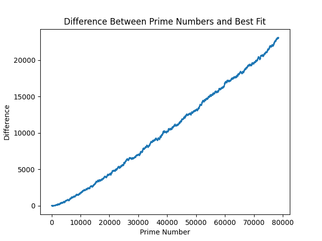
Difference in prediction and primes of x*log(x,y) for 1 million primes

Remember that this is still with our y=6.84 value we found through fitness. If we go back and try to fit a best y value with our million smaple-set, we get a new fitness value: y=56 brings us to a error rate of:

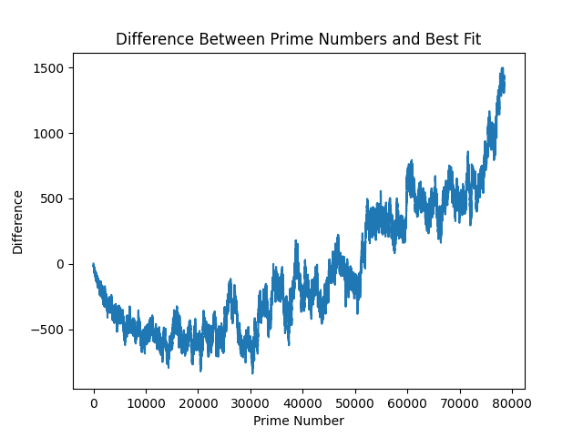
Difference in prediction and primes with a new fitness

Going down this rabbit hole, similar to plotting the minimum value of y-values above, moves us into overfitting territory. What strikes me (and I don't want to get narrowed down on this idea), is that the new goal should instead be as follows:

Attempt to flatten this curve at large N. If there's a way to flatten this, and get differences closer to 0 as N rises higher and higher, then the model difference is a more attackable problem.

From here, as I've fixed the equation modeller also, I am going to test some more brute-forcing equations to see if I can find anything else to help this adventure.

Equation Modelling

My knack is that our equations are platonic (Talebian term) in a sense that we're modelling in a standard logical language, something of which might require complex, or non-platonic randomness and chaos. This is just a hunch - but at the same time I am really shocked at how well a basic equation can model the randomness of prime numbers. I do not understand logarithms in my soul, only on the surface, so this is an area I am going to look further into.

Equation Interfacing

There is an existing complexity which I accidentally noticed - testing at x=2,4,6 rather than x=1,2,3 is inherrently weird - but worked well. It's possible that a rate change in the x increment is a meta-equation which can reduce complexity in the equation itself, and also lends itself to a higher rate of experimentation.

I'm considering, though find it hard to grasp, building a more dynamic interface which is able to accomodate this. At the moment, I am using the following lines to for example bake in a 2,4,6 step in x values:

X_INC = 1
X_TIMES = 2
...
for x, _ in enumerate(primes):
   x = x + X_INC
   x = x * X_TIMES

By creating an equation to build X values (2x, x^2, or otherwise), this starts to give light to the idea of combining multiple series of equations to solve the problem. This might be unnecessary, as this can also be represented as:

(2 * x) * (log((x*2), 7)) at x-step = 1

Which provides the same output as stepping by 2. By being able to accomodate this structure (which cannot currently), this can be tested for efficacy before adding this complexity.

I've done this by adding another set of options for the expression builder with:

ERROROUS_ADDITIONS = [
   "log", # 18
   "sin",
   "cos",
   "," # 21
]

Which can embed the above function on x-step=1 by embedding the following:

ex_str = supplement_ops(
   [6, 2.00, 2, 10, 7] + # (2x)
   [2] + # \*
   [18, 6, 2.00, 2, 10, 21, 11, 7] 
) # returns: "(2.0*x)*log(2.0*x,y)"

The question then becomes:

Is the problem space better if fractionated into multiple equations, or is it better to attempt to build a mono equation?

And I have no idea.

When running this modified generator with more possible equations, and also a higher chance of a failed equation, some equations and their 1,299 fitness are:

Cut down length of equations from 100 to 25, since most equations so far have fit there. I will lift this in the future to not be fooled by randomness.
((x*sin(sin(1.1717823427685636)))*log(x,y)) at y=2: 17,323 fitness (great one-shot result before optimisation)

((x*sin(sin(1.1717823427685636)))*log(x,y))

Taking this equation, and y-fitting, we find it gets most comfortable at y=2.0026 (14533.53 fitness). Narrowing down further, we get a miniscule smaller at y=2.002564 (14533.16 fitness). Tiny difference in a higher precision.

At 1,000,000 primes, we have the following fitnesses:

Prior x*log equation fitness: 811,473,649
New sinusoudal fitness: 511,239,573

New sinusoidal plotted:

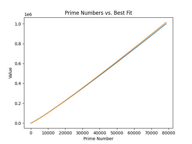
And difference:

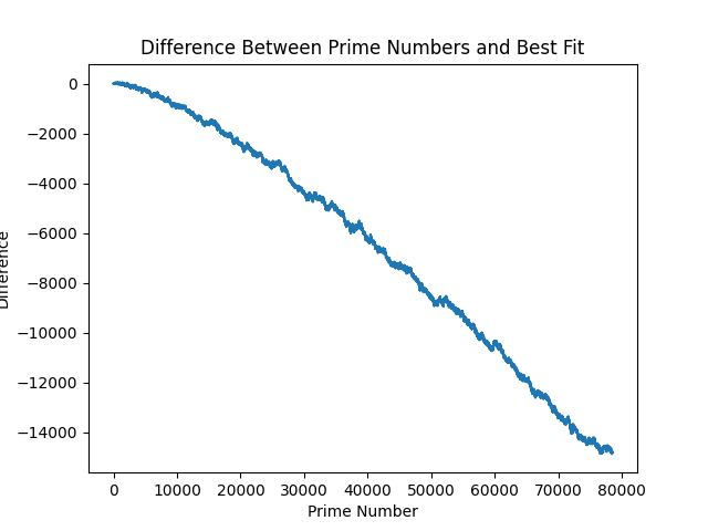
As you can see - the difference is negative (grows larger than the primes at scale).

What I feel is a property for a prime number expression or equation, is something like:

It cannot be fitted to a certain area (first 1,229), and then expect that fitness to scale further to a larger area.

It's also noticeable the constant in this equation: 1.1717823427685636. This is actually a constant inside a sin(sin(...)) function, which then resolves this constant to 0.7964759083371821. The simpler equation is then ((x*0.7964759083371821)*log(x,y)), which brings us right back to the start.

I was fooled by randomness - and tokens.

(I was going to remove this section, but I am committing to the format of a journal, to outline the process and how it felt to move from each step to another.)

This is bitter-sweet - and let me explain why.

Multivariate

I was considering whether or not multivariate (beyond X and Y) could help in the complexity of primes. In my handwritten journal, I wrote the following note:

(With the broader equation builder, which can facilitate 2x and log((2x), y) for example) we have a broader dynamic chance. For example: we can multiple x by 2 different equations, OR constants. They are both variables.

What I meant by this was that with the broader equation builder - although it operates with a much larger error change, the "possible" space is larger. Like monkeys typing randomly to make shakespeare - if you restrict the alphabet or wordlist, you might miss dickinson.

This is an immediate validation that there is more possible variation, since we've created a multivariate example within ~15 minutes of running this random generator - which is more fit to the prime numbers than previous models.

I think this comes together well with the above next steps in my mind.

Optimising the Constant (C)

When optimising the constant, it can be brought down with the following slight digit changes:

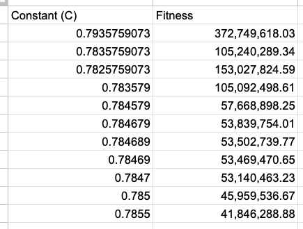
This creates the difference from the primes of the following:

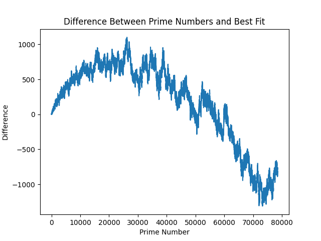
Next Steps - Optimising, and Grouping Primes

Next ideas:

It may be valuable to tweak this 0.7964759083371821 constant in the modified equation WITHIN the groups, to find how this adjusts.
It may also be valuable, once this is worked out, to check at the optimal fitness as the groups scale. We can break up the 1,000,000 primes into groups of 1,000 groups of 1,000.
Modelling and plotting these might provide an interesting scale that can be seen - or some randomness that cannot be tamed. We'll see!

With optimising, there is a possibility that X, or other values, might need to be adjusted across a separate equation. First, I will try adjusting the separate constant.

Nearness

Something I have noted when looking at the difference charts, is that there seems to be some form of nearness bias, or gravity. What I mean by this is that no subsequent "draw from the bag" for the next difference value is radically different from the previous difference. In fact, they seem to cluster, and follow trends, or mean-reversion. When I take the second-delta of the difference (delta of the difference), we see this chart:

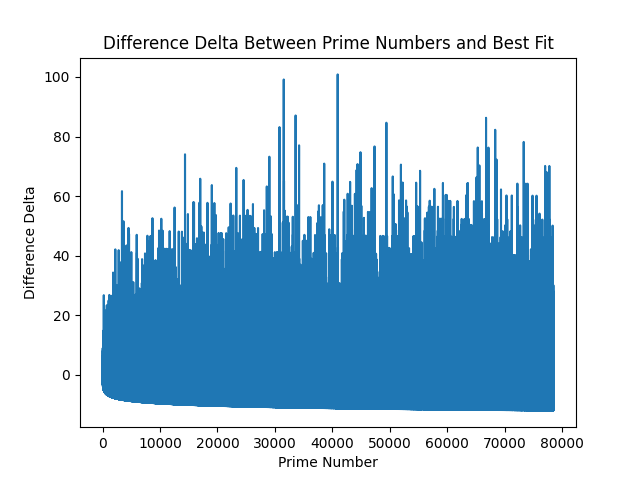
(25th of October addition: I was thinking this yesterday, and forgot to write it - the above looks like a very fuzzy positive upside, with a very predictable downside variant - as it's following some sort of negative curve.)

This displays two properties:

Positive values could skew further and further into infinity.
Negative values seem to follow a inverse log asymptote (if that makes sense).

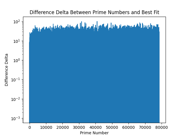
If we then use log scales for the Y axis of the delta difference for the first 1,000,000 primes, we see:

And zooming into the first 250 WITHOUT log of the above series, we see:

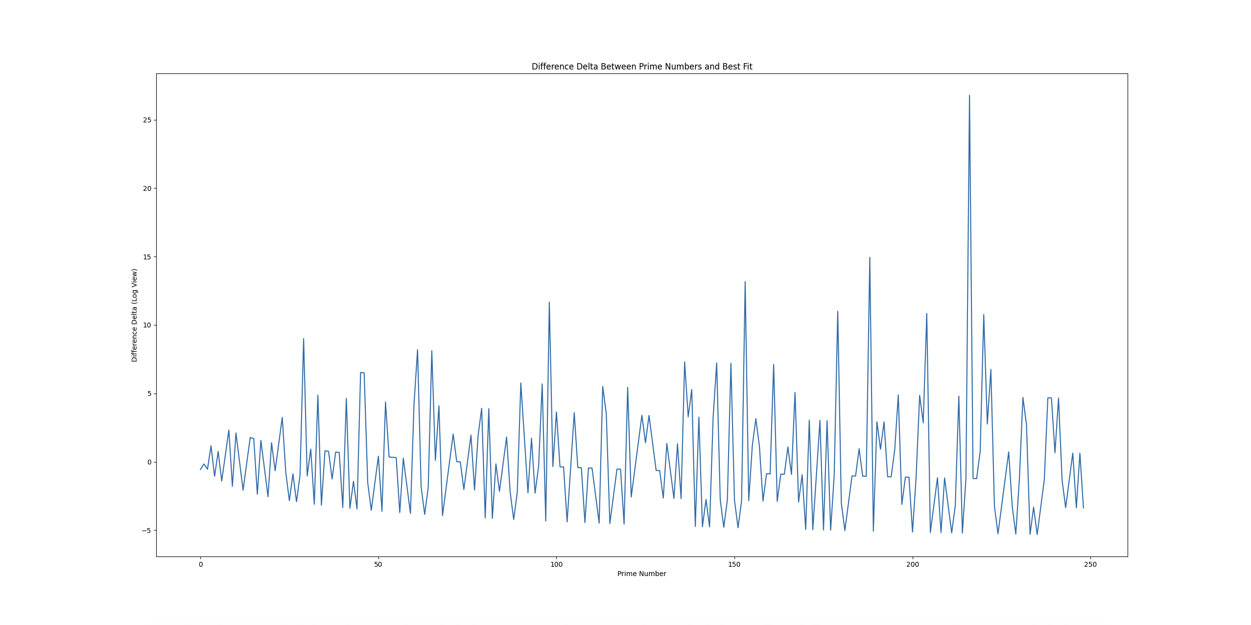
First 250 primes NO LOG difference delta

(For this one, I recommend right-clicking, and open in another tab, as it's better to see it on a larger device.)

With LogY:

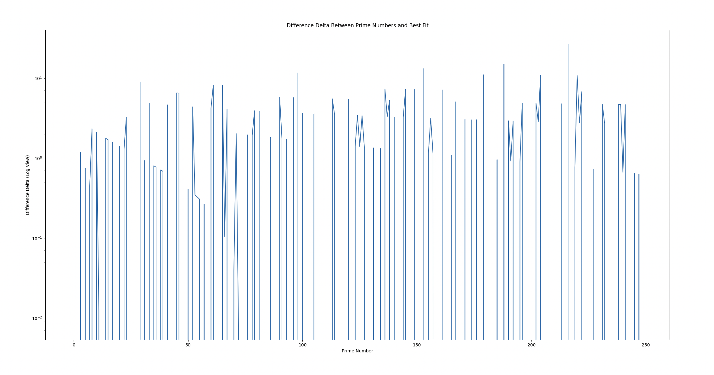
Both show interesting patterns, though with LogY it seems fuzzier locally, whereas at scale, it seems as if there's a bias towards negativity. The problem then might simplify into: trying to balance positive difference and negative difference at scale, which we might solve with tweaking in groups.

For the nolog plot, the bottom line of the pattern looks like a plot, as well as the band above it looks like it follows with constant fixture.

I want to remind myself and readers that it is not my job to reason about this crazy randomness to solve the problem - because I cannot plan the answer in any way. It's too wild. So, I will keep stepping forward cutting up little problems into heuristics, and trying to reason about the properties of what is occurring here.

Group Fitting

Fitting to the groups is an interesting engineering problem. On one hand, we're aiming for the most optimum fitness. On the other, I am thinking this:

Prime numbers are tricky, like their distribution. We may want to do vector analysis on the series of multivariate values, rather than simply going for the single "best" value for each group of 1,000 primes. There might be a slightly less optimal set of values which fits the group, but it might correspond to a better trend in long-term performance. We're looking for signals, not just noise - but we'll start with the best in the groups first to see if there's an interesting trend there.

As I do some testing in the background, I will call it a day. Great progress, and lots to ponder on. I want to take all of this expansive properties, and compress it down to keep it simpler.

25th of October, 2024

Refresh, Review, Reprise, Refactor?

Alright - a lot of surface area was generated yesterday by narrowing down to trying to do overfitting to the prime curve. We know that local optimisation of fitness does not equate to large optimisation and fitness. What does this mean then? Are we destitute to be stuck in a machine-learning-type overfitting or underfitting problem? We can't be probabalistic about this, as we're wanting to work out what's going on here. Even a tiny miscomputation in the algorithm equates to an enormous deviation, as per our chaos, and three-body-problem discussion. With this in mind, it's further clear that optimisation is not aiming to "crack the primes", it's rather an attempt to review the outputs, and see if we can understand the system, and trajectories, to build something purer, and closer to the prime curve.

I think a brief refactor may be of value - to get components into a clearer picture so I can move forward with more testing.

Property: Negativo Contro Positivo (Negative Versus Positive)

If you look at the above Difference Delta Between Prime Numbers And Best Fit (24th of October), I added a note that I remembered, where it looks to have a predictable volatility: volatile upside (positive), and a predictable downside (negative). A future experiment I will do will be with the actual data points, in a more frequenty analysis format.

Precision On Single Primes

I had an idea when looking at groups, and considering looking at smaller groups - like 100, instead of 1,000. Out of nowhere, the idea popped up:

What if we look at the values required to get perfect precision on a single prime? In other words, let's try tuning to a group of 1, where X stays stable, and we modify Y (log of), A (coefficient of x * ... term), and B (log(x*B) coefficient).

By doing this, I quickly experimented and found there were interesting trade-offs with precision. For the first few primes - I could get good precision. With the intervals I was stepping (0.1), that quickly started to face at higher primes, like the 100th, and 1000th.

I then thought: what if I could eliminate multivariate? Where I began to simplify the equation by removing variations on single components.

I removed A variations - precision was still there.

I removed B variations - precision went away.

I added a higher precision to Y, and it came back. I had to move it to a 0.00001 step interval for Y, for it to return to finding a close-enough (within 0.00461 precision) result to the prime, with a Y value of 2.39269. This is fascinating!

When I do the same for the other variables (singling them out as being adjusted), and Y=7 (how I found this expression first), the following properties occur:

(101th Prime 547)

A: 0.0011 precision at A=2.283520.
B: incredible precision at B=373.763.
Y: 0.000735 precision at Y=2.344690.

(501st Prime: 3581)

A: 0.00131 precision at A=2.237360.
B: incredible precision at B=2191.157000.
Y: 0.00434 precision at Y=2.386280.

(1001th Prime: 7927)

A: 0.009994 precision at A=2.23048.
B: 0.000691 precision at B=4920, and incredibly close precision at B=4920.007.
Y: 0.004606 precision at Y=2.392690.

With this in mind, it's important to realise that we can likely fit any equation to the primes in order to manufacture a series. Though, if we were doing this trivially, we'd likely get something very close to the prime numbers in terms of relationship to the values.

With the above, we can see that the underlying equation has values which show some sort of pattern (the XX in 2.XX for A may for example be a prime number in disguise, and fool us), and we can also see B grows as the primes grow (it may grow by the prime number increase). We can also see that Y fits this above-2 value, and grows positively (from sample data so far, whereas unlike B in our sample data, which we do not know its growth yet).

Either way - we have some more exploring to do, and I'll begin to work on a precision finder for each of these value, and I feel as if this was a very interesting find for the equation. Off to data mining so we can plot these values over the primes!

Shower Reflections

I just had a shower (not necessary for you to know), but during the whole shower I could think of little but this problem. I spend a lot of time working in data, and there are periods of enjoyment and creativity, but truly nothing compares to the unbounded, self-fueled creation space, over anything else. I realise I enjoy, more than anything, chewing on these tough ideas that just don't give. I want to get to a place where this can be my main endeavour, as I do not even know what problems are out there to look at and help solve.

I see two current "next steps" that stand above the rest of the many ideas I am having for this prime problem:

Building a streamlined per-prime tester, precision finder, and data collector.
Investigating, with frequency analysis, the positive and negative differences with a static value over time - to see if there are relationships in the positive versus negative values, as I pointed out in the "volatile positive values, predictable bounded negative values", and seeing if there is some sort of relationship there in frequencies / samples.

Next, I will work on data mining, and move into the positive & negative potentially as well, to gather more properties.

Building The Prime Miner

Some following thoughts:

We want to do two things: find the best value to fit the equation to the prime, and we also want to capture the value range which results in an output which rounds to the prime. This is so when if we're fitting an equation to this, we can look to fit to the range, as well as the most precise, to see if there's a difference.
Idea: When we find a best-fit range of values (values that would result in a value which is roundable to the prime), can we find a whole fraction which fits that value? If so, can we find a pattern in the whole fractions, or the possibility of a whole fraction-ness?

Reviewing The Results

It's a slow process, and I've only done the bottom 1,229 so far, so I do not want to get ahead of myself. It is utterly fascinating seeing this pattern. I am going to go for a walk, let it run a bit more, ruminate, and come back to start analysing the data.

When A lowers from its prior most optimal value, Y-optimal raises higher for it's optimal value to arive at the prime.

25th of October, 2024

I've not spent a lot of time on the problem today in terms of the hard stuff, but I have been thinking about it quite a bit. The data miner has been built, and I am going to do some analysis on the data, as well as compute with the optimal values to make sure I've got the resulting values being parsed correctly.

Below is a plot of the fittest Y value to get the prime at N for the equation. As a reminder, I will include the equation which is being optimised (without the other variables) above each plot. Below is the Y-plot:

Y-Fitting: x * log(x, Y)

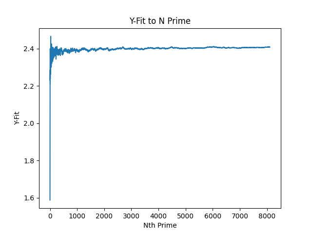
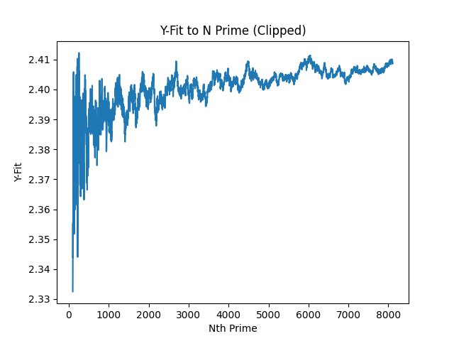
I was going to remove the first few primes from the sample to scale it better, but I thought it would be useful to see it how I see it - like a wild plot which I can't remember the name for. x sin(x) (since it's sort of sinusoidal)?

With the front clipped (so you can see the smaller segment better), we get this:

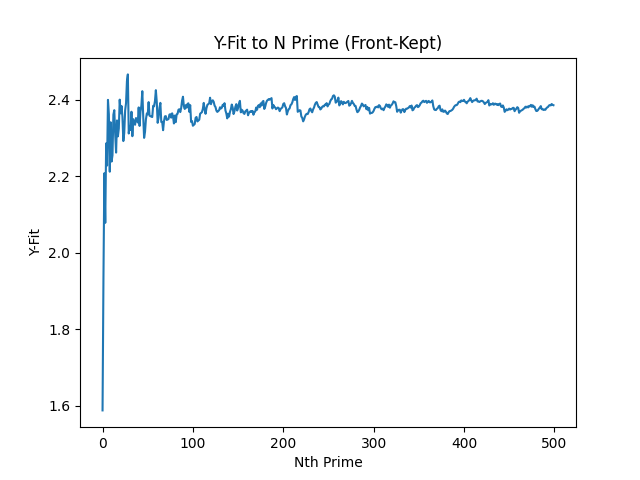
And the first 500 primes:

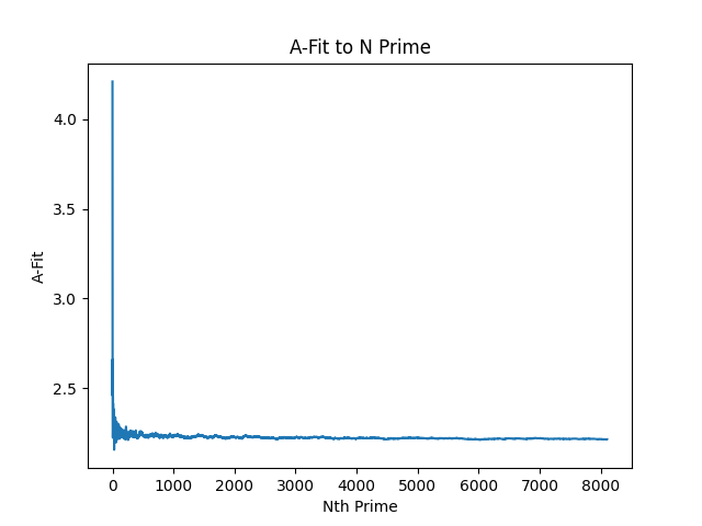
A-Fitting: (A * x) * log(x, 7)

A-fit macro chart:

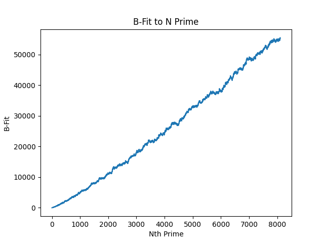
B-Fitting x * log(x * B, 7)

B-fit macro chart:

There's a lot to unpack here

The above are quite thought-provoking.

Y-fit seems to bias negatively from the longer-term mean in the sample size.
A-fit seems to bias positively from the longer-term mean in the sample size.
B-fit has a positive, growthy curve, but looks light it might be slightly curving.
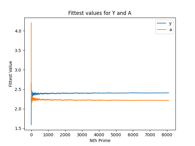
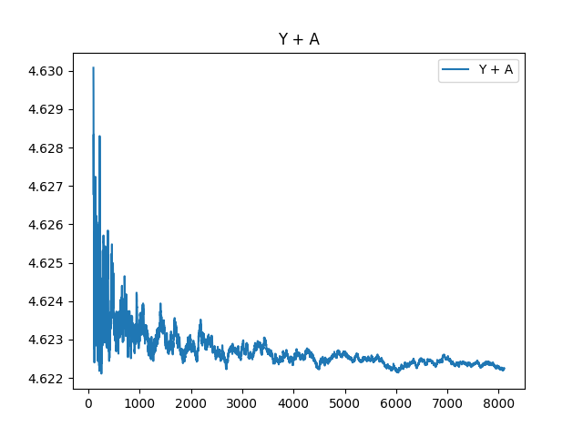
I'd like to look at A+Y in a chart, to see how they behave (on initial watching, I did notice that as A increased prime-over-prime, Y tended to decrease, so this might be interesting to look at).
Y-fit looks stable at ~2.4, but might be ever so slightly increasing.
The further you go into the primes, the slighter the precision adjusts
B going up and down is quite fascinating: this is because it's known we're looking at an ever-ascending prime series, but these whole numbers for B can be better fit for future primes at a lower value. The B-fit was stepped by an interval of 1, since it was a very high figure to reach compared to the sensitivity of A and Y. This might reveal something about the weirdness of primes: what we're observing here is that some future primes are better fit to lower B values, although there might be some series of compatible B-values which have a more consistent looking curve - since the range is wide in B values which can predict the prime. This needs some more thought, as I'm struggling to wrap my head around it.
A further variable I have not controlled yet is X. I am curious how, if we keep the equation at x * log(x, 7), what X values are required in order to hit the primes. This is a different way of looking at things, since it looks to a fit curve, then asks what the input is for the N. So it's more like trying to find an equation for the right X value on the curve.

Let's start by looking at the overlapping Y and A charts:

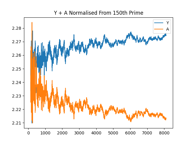
And clipping the fronts, and standardising the difference from the first value to start from the same spot:

And Y + A plotted from the 100th prime:

And finally, the delta between Y and A:

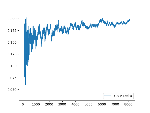
A few additional thoughts:

A and Y fitnesses seem negatively correlated, though there is a bias for Y fitness to slowly grow out of this correlation over the long-term in the sample we have.
There might be a better way to understand the gap between these values, to understand their distance over time better?
A fitness seems to trend negatively, while Y trends positively. Remember: these are the optimal values to get as close to the prime as possible, which could be a bad anchoring point to center on. This is because from the data mining I did, there is a range of values which the output can be rounded to get to the prime number (found using abs fitness < 0.5). I will do analysis in the future on the ranges.
If it was a choice between trying to pinpoint A fitness (trending negative) and Y fitness (trending positive), it seems an easier problem to wrangle to-negative complexity.
A must negatively be approaching some infinite bottom point, as the (x * A) component cannot reach 0, as it would no longer produce a positive prime number.

Confirmation Bias

We're looking at a small sample of data. It's possible that there's a breaking point where we reach a threshhold, and things adjust. I will aim to keep researching this research space to better understand it, as it feels like the right pathway (understand what's infront of me and already difficult to compute, then go there).

Y-Fit Deltas, and A-Fit Deltas

(The below are all from the 100th prime to be able to better visualise the pattern on a smaller figure.)

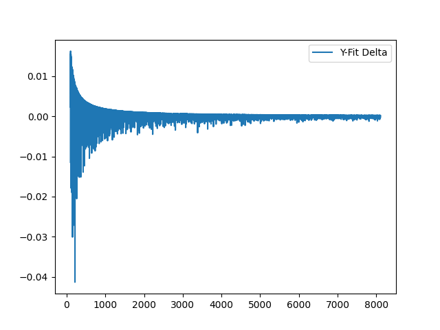
Y-fit delta between each value adjustment:

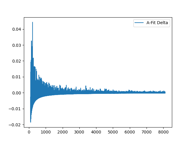
I just had a mind-melting moment. A true "WTF?" when plotting the deltas between Y-fitness and A-fitness.

I don't really know what to make of it yet, but this idea of capped upside and downside is returning.

Take a look at the rate of change (delta) for Y-fitness:

And A-fit deltas:

And now, overlapping A and Y deltas:

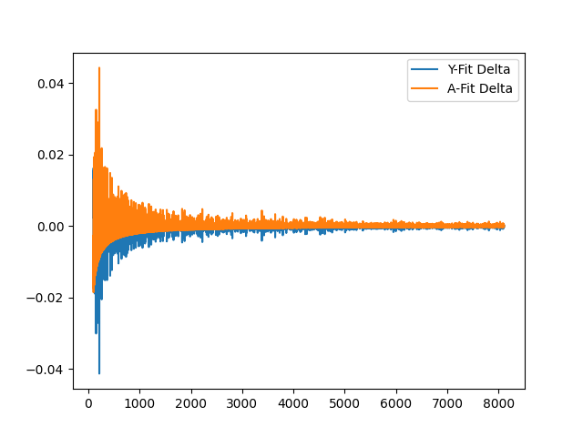
I'm sure this is just bamboozling once again, but I feel as if it describes the slow tilt-up with any attempt at fitting the prime curve. We see a semi-related, semi-correlated inverse relationship, though it slightly deviates over-time.

(Added as a remembered previous thought: is it possible to then define the value Y or A will be, by using this positive capped value, and negative capped value?)

This makes me want to investigate the delta of the difference between Y-A chart to see what manifests there:

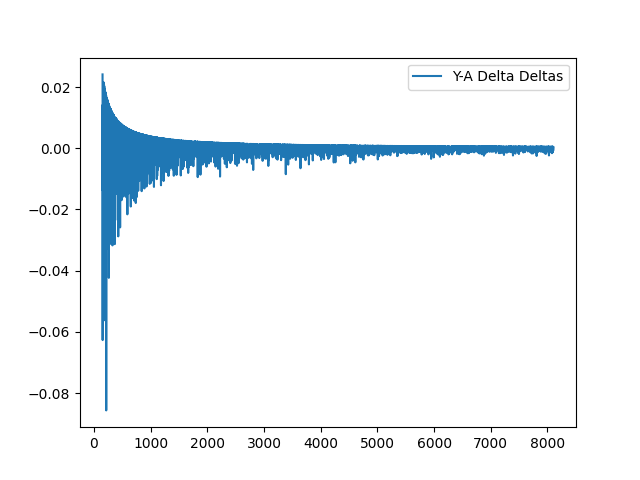
I saw this here, but I did not notice it in the above charts: they seem to also have a capped upside/downside, but it tends to have more volatility also.

Zooming in, the choice of up or down seems random. I will reflect on the above for a while, but I wanted to do some frequency analysis to see if there's some pattern in the delta's movement. Easier to understand, there is:

The size of the move (?)
Whether it was a positive domain move, or a negative domain move

And, if (2) can be solved, it all helps in the grand scheme.

So, I've done some frequency analysis before I go to bed, and here is a positive value for the number it was positive, then negative for how many it was negative for:

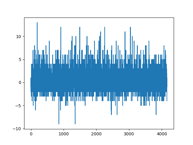
Y-A Difference, Delta, Frequency Analysis

And, the clipped first 75:

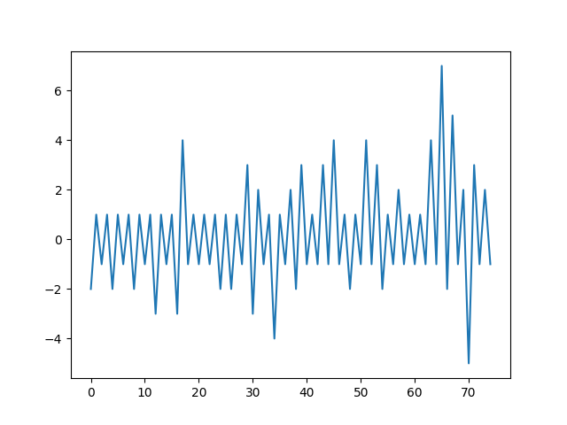
Y-A Difference, Delta, Frequency Analysis upto 75

And I leave you with the above for this day at 11:45PM. Some further frequency analysis on the pulls might be of interest - for example - by checking the frequency of 1's, 2's, etc - maybe a gaussian will emerge? I'll believe it if I see it!

Further, tomorrow, in my reflection, I want to bring this back home and ground it back in the equation, so we're able to understand where we are. I do not want to go down a rabbit hole, so it's always important to re-ground on where we are, and what we have so far.

27th of October, 2024

G'day. I just played Bingo for the first time at the Merimbula RSL. It was definitely an experience. In the first half, it was quite fun due to the novelty. In the second half, it steadily got tiresome mentally fixturing on sheets of paper and numbers, even as a 23 year old casual number enjoyer.

What was incredible was my friend Vanessa won, but we did not know we had to call it before the last number (which won the card) moved on. We almost won $50, which was unfortunate, but anyway - life goes on.

Anyway. I was thinking about how I was discussing the two problem spaces above (solving the direction, and amplitude, are two separate problems), and how:

If it were possible to solve the directional frequency problem, we would accidentally discover the bounds for where the prime will fit in the equation. This is if we are doing it in an iterable way (solving Prime 1, Prime 2, etc).
For instance: if we knew the next Y-Fit value (bounded positive side, see Y-fit delta above) is going to be positive for the next prime, then we might be able to know the bounds for where the value can lie. I don't fully understand this relationship yet, but it could be valuable.

Optimisation

The next stage to me, is data collection. I want to optimise the data collector / miner, since that has proven itself a valuable component to the research. Time to supercharge the miner.

Upcoming Travel

I am travelling from the 29th of October to Bali. So updates will be a little less frequent, but they will still occur. Over my flight, as this is an internet-less problem, I'll be able to do experiments.

Work: Optimisation

I've written an optimised Y-fit optimizer. I've decide to set the cutoff at an absolute fitness of 0.001 for good measure.

Before, I was doing 1,000,000 tests every iteration. Now, I've tested on the 201st prime 1,227, and it took 187 steps in order to get the right Y-fit value of 2.3805784.

This is hilariously faster (I was not trying to tweak performance), and is 5,348 times faster. The other positive to this approach is that it does not assume a step interval, so it will always attempt to narrow down on the correct value, no matter how deep it has to go to get there. These are two big advantages.

(I've also made it select the just-over-prime value, rather than getting a few results below prime then rounded to prime, for consistency.)

The downside was the engineering was hard for my mind to wrap around. I need to work slowly to get the tools I need.

I've run the fitter on ~72,000 primes (first 1,000,000), and it completed the fittest-Y within < 10 seconds (9.63s). It was expected to take ~20 hours using the prior method, just for the Y-Fit values (multiple days for Y, A and B computations).

Here is a plot of the up-to 1 million primes:

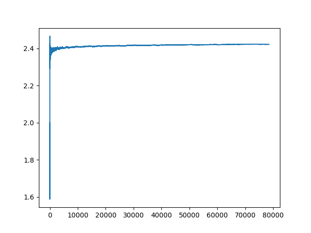
(I will fit this to a prime generator also, to extend the plot further and further out, and look for a larger prime set.)

This further provides more experimentation allowance, since I can now adjust multivariate values (Y=7 for A, for example), to see what can happen (can adjusting Y reduce volatility in A, or increase it, or nothing?), and I can also compute the fitness values much quicker.

At a minimum, I feel as if I am answering the confusing questions I had in 2022/2023 regarding why the heck do you fit a equation to the primes at 0-10,000, for it to all fall apart. There are still many questions and tests to do, but this is a fascinating sub-area of exploration.

What are we fitting?

I had the thought to what if we're over-fitting the values. What if this just represents another representation for the prime in a hidden way? I think that could be a piece of it, though I tried running the Y-fitter on ascending X values, trying to fit the X output, and it's a linear curve like Y=X.

So what we're currently tweaking is:

Assuming a linear X (1, 2, 3), what log base (Y) do we need to get the Xth prime?

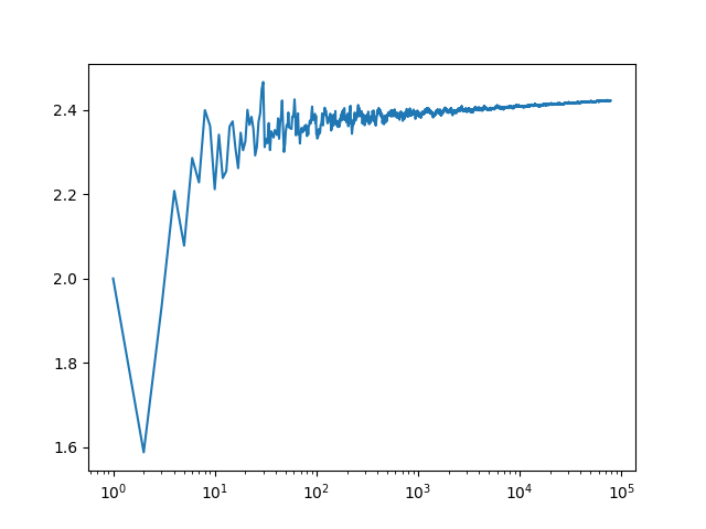
1m Y-Fit Primes Log

Below is a figure of the primes Y-Fit with a X-scale which is logarithm:

28th of October, 2024

Hello! I'm in Sydney at the moment, preparing to fly to Bali tomorrow with my partner.

I've plugged in the 1 billionth prime (22,801,763,489) into the tweaker for Y, and got a Y of 2.4814544815638517. For the trillionth prime (29,996,224,275,833), the Y value is 2.5121776604449253 - cracking 2.5!

For A, on the other hand, the A value for the billionth prime is 2.141080625935799, and trillionth is 2.112479195277878. We're seeing Y go up, and A go down. I'm presuming we can reach infinitely large primes if we're able to crack this, but the race to infinidecimal on the other side will make it challenging.

29th of October, 2024

This means that:

A-fitting: negatively biased. Y-fitting: positively biased. Y-fitting growth overpowers A-fitting negative growth.

Per x * log(x*B, 7) being fit, it's quite linear, and over time gets closer to linearity. At the start it's quite volatile, and over higher N's, it begins to look linear. Here is a plot with X and Y log: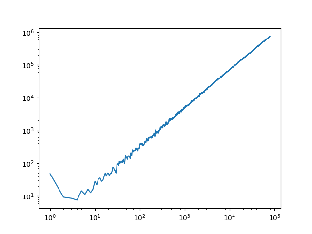

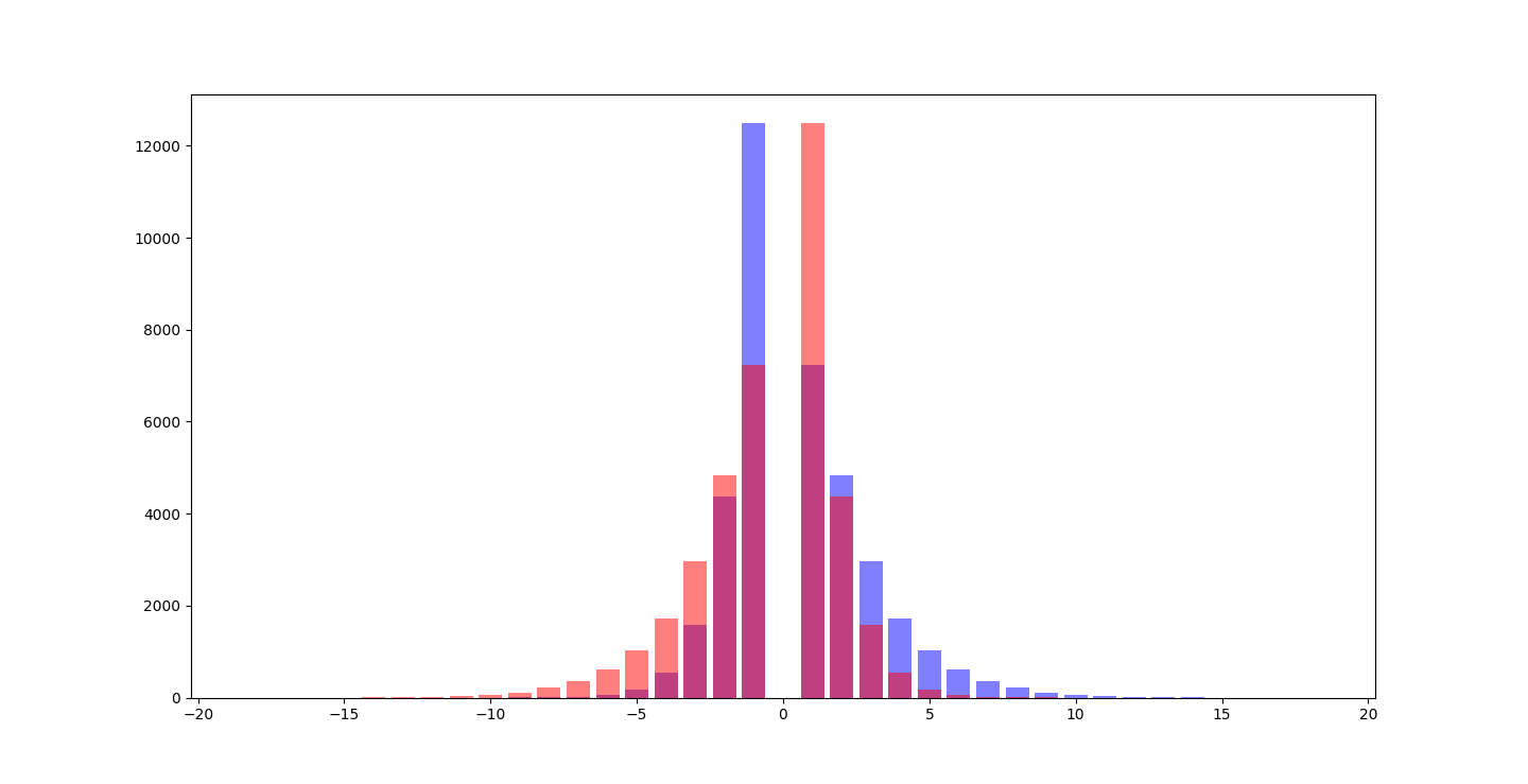
Spot The Gaussian

Y-Fit series delta, with trend of negativity or positivity.

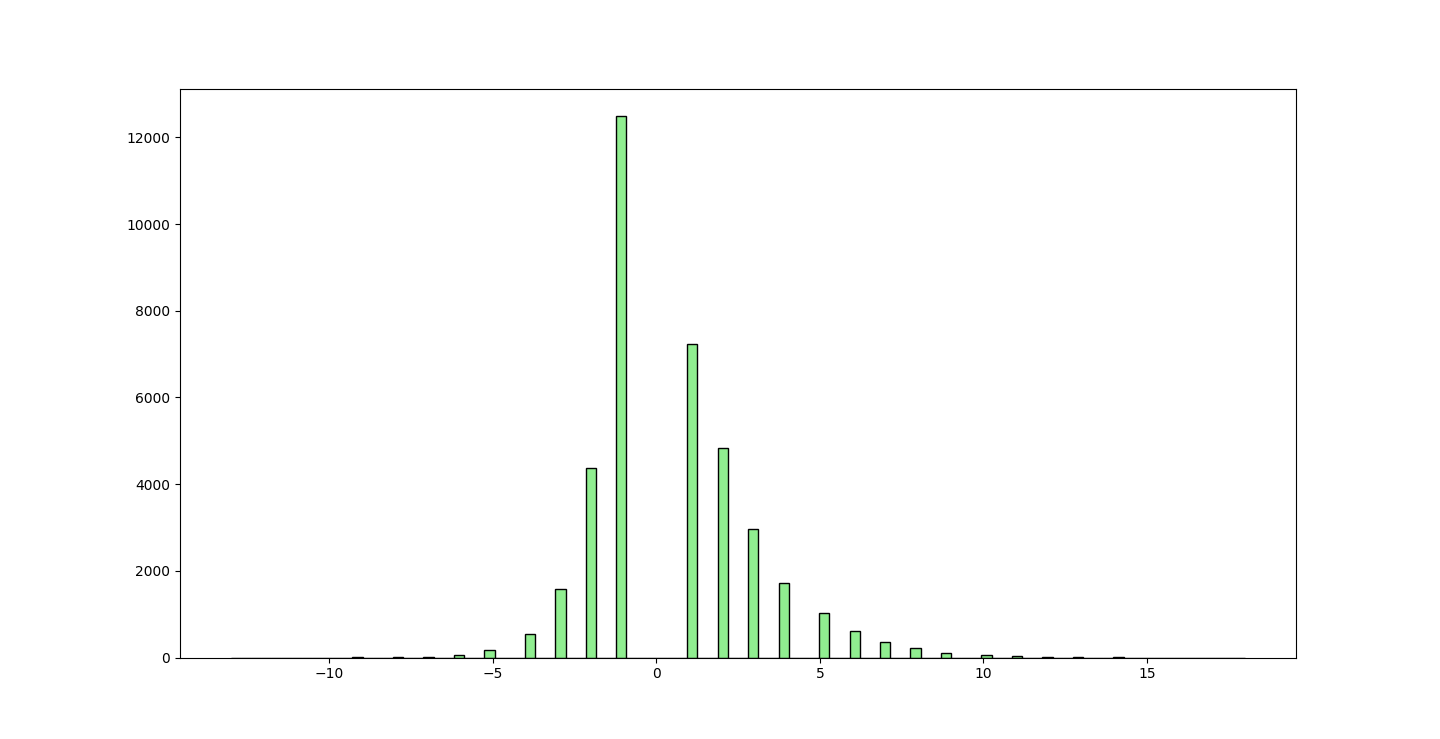
When we do the A-Fit reversal trend (the frequency of how long a trend is negative, or positive), we see:

A bias of a higher single frequency towards the positive, rather than negative as the Y fitness deltas trend in.

Overlapping:

3rd of November, 2024

I've been enjoying Bali for the last few days, drinking Bintang's and having a good time. I've thought over this problem for a bit, and also spent some time doing some statistical tests that ChatGPT helped me understand. Some examples are:

Augmented Dickey-Fuller (ADF) test: data is "static" (mean does not adjust over periods) on Y-delta set
Kolmogorov-Smirnov Test: does not indicate a standard distribution, on any of the datasets.

As I've been going deeper on looking into standard statistical methods to analyse this data, I feel as if I am moving further from what has gotten me to this position in the first place. It was interesting looking at skewness, kurtosis, mean, and standard deviation, and I know enough Talebian remarks to know to keep tinkering, as well as look at the conventional knowledge when necessary. To summarise: it feels like more noise, than signal, using the conventional statistics, and the unusual names (no hate to the authors - their work is valuable, but I don't want to keep the cool word "Kolmogorov" in my head while I am working on puzzles).

I also looked at the X values which fit to the curve, which I will do more research on.

From here, I want to look at the following:

Using different ways of looking at deltas: looking at not just difference, but percentage changes, and investigating other ways of looking at data deltas.
Looking more at the pseudo-gaussian-looking distribution of the positive and negative periods.
Looking into the amplitude, and seeing if there's any pattern there.
Looking at the Y values and their neighbours, to see if there is any need to actually adjust the Y value between primes. If there are trends where there's no need to shift the Y value, I want to know how long for, and plot it.
Group values, and see if there are any trends. I've noticed in the Y-fit difference delta-delta, there are interesting looking pairs of Y values which follow an unusual trend of 3 positive Y's, then 3 negative Y's, as well as values that are very close together.
Look at the x-fit values of the equation.
Look at potential ways of classifying volatility of series to indicate how volatile the series is (this is something I notice when I dig into the delta delta delta ... delta series of a series - the prime series has no "floor" of volatility, but there might be a way to classify if the series is more predictable than another) - cumulative error to the mean, or something?

Below, I will begin to refactor, and get things back into shape.

MAD, CAD, SAD

A ChatGPT discussion on using MAD, and CAD, for looking at volatility.

One candiate for classifying the volatility of a given series, might be to look at the series MAD (mean absolute deviation), and CAD (cumulative absolute deviation). This can be done by taking the mean of the series, then summing the absolute error from the mean. The mean can then be taken by dividing the cumulative value by the length of the series.

To normalise across multiple domains, we'd need to normalise in another way than we do currently. When doing N difference-deltas, the values change wildly. This fits perfectly into looking at new delta formats, of which I believe percentage deltas might be a valuable way to look at looking at the multiplicative changes, as well as try out our new error reading.

Without normalisation, and instead using differencing, we see this trend (i=0 is without a delta):

0: Cumulative Absolute Error: 412.22664980219366, Mean Absolute Error: 0.00525142869630044
1: Cumulative Absolute Error: 12.245210541465505, Mean Absolute Error: 0.00015599590483032107
2: Cumulative Absolute Error: 18.664078700445422, Mean Absolute Error: 0.0002377710800607111
3: Cumulative Absolute Error: 32.958655522779026, Mean Absolute Error: 0.00041988222845758895
4: Cumulative Absolute Error: 60.773011335477, Mean Absolute Error: 0.0007742376657512292
5: Cumulative Absolute Error: 113.57485893271077, Mean Absolute Error: 0.0014469425163098702
6: Cumulative Absolute Error: 215.91894630252366, Mean Absolute Error: 0.0027508401659088726
7: Cumulative Absolute Error: 409.19805442259155, Mean Absolute Error: 0.005213311773612131
8: Cumulative Absolute Error: 786.7621861772942, Mean Absolute Error: 0.010023725139219038
9: Cumulative Absolute Error: 1502.9569714895779, Mean Absolute Error: 0.019148631929182057

With normalisation using multiplication, we see:

0: CAD: 409.9202814226476, MAD: 0.005222380102972903, Mean: 2.416269020020983
1: CAD: 4.92239738463249, MAD: 6.271209020830657e-05, Mean: 9.978725243008389e-07
2: CAD: 321885.9494663943, MAD: 4.100928125089449, Mean: -0.8927910663009873
3: CAD: 463436296524.5065, MAD: 5904399.242253961, Mean: -2877658.1039074394
4: CAD: 888685701093.1577, MAD: 11322423.538243068, Mean: -225435.23483871602
5: CAD: 1060074814545.8591, MAD: 13506202.40732162, Mean: 2256839.6436438635
6: CAD: 5927620458707.524, MAD: 75523595.73824328, Mean: 33912450.2932923
7: CAD: 24671665846026.152, MAD: 314344798.38478273, Mean: 119619755.40753777
8: CAD: 35126696621113.21, MAD: 447559363.2045754, Mean: -206655960.85012862
9: CAD: 3927080975254230.0, MAD: 50036707803.57053, Mean: 24907161415.62895

So, we do not get a better read of volatility - or we see volatility increase at depth.

And with a logarithmic delta:

0: CAD: 409.9202814226476, MAD: 0.005222380102972903, Mean: 2.416269020020983
1: CAD: 1.0701098485086775, MAD: 1.3633361979673728e-05, Mean: 1.5971013924538176e-07
/Users/jackhales/Dev/prime-number-research/primes/precision_miner/uq_analysis/deltas.py:29: RuntimeWarning: invalid value encountered in log
  d = (np.log(s1) / np.log(base)) - (np.log(s0) / np.log(base))
2: CAD: nan, MAD: nan, Mean: nan
3: CAD: nan, MAD: nan, Mean: nan
4: CAD: nan, MAD: nan, Mean: nan
5: CAD: nan, MAD: nan, Mean: nan
6: CAD: nan, MAD: nan, Mean: nan
7: CAD: nan, MAD: nan, Mean: nan
8: CAD: nan, MAD: nan, Mean: nan
9: CAD: nan, MAD: nan, Mean: nan

Which makes sense, since log values are small.

With 1 + x in the log delta, we can go a little deeper:

0: CAD: 409.9202814226476, MAD: 0.005222380102972903, Mean: 2.416269020020983
1: CAD: 3.472213248986966, MAD: 4.423652409146064e-05, Mean: 5.161604338429603e-07
2: CAD: 5.177304217502216, MAD: 6.596048231647372e-05, Mean: 2.293725237169149e-07
3: CAD: 8.989736292023549, MAD: 0.0001145335239141753, Mean: -8.448973252904579e-07
4: CAD: 16.40981409444938, MAD: 0.00020907151440902174, Mean: 1.7755820384512643e-06
5: CAD: 30.56834706119753, MAD: 0.00038946523113337966, Mean: -1.9607584593122482e-06
6: CAD: 58.58615471516942, MAD: 0.000746444057170858, Mean: 9.58898120589133e-07
7: CAD: 114.98918793785522, MAD: 0.0014650917098317714, Mean: 7.707736901095848e-06
/Users/jackhales/Dev/prime-number-research/primes/precision_miner/uq_analysis/deltas.py:31: RuntimeWarning: invalid value encountered in log
  d = np.log(1+s1) - np.log(1+s0)
8: CAD: nan, MAD: nan, Mean: nan
9: CAD: nan, MAD: nan, Mean: nan

Then doing log on the first delta, and absolutes, shows nothing significant but an increasing CAD over time.

Although this has yielded nothing of substance (the CAD seems to grow at a multiple as we go down layers, that's about it), this does showcase a good way to gauge the error rate over time. It also indicates that the least volatile layer to look at is the first delta. This might constitute another principle, as well as an important thing to find - a series where the volatility shrinks at delta depth.

In the series x^2, the difference CAD at depths would be:

N = 1 2 3 4 5 S = 1 4 9 16 25, Mean = 11, CAD = 10+7+2+5+14 = 38 D1 = 3 5 7 9, Mean = 6, CAD = 3+1+1+3 = 8 D2 = 2 2 2, Mean = 2, CAD = 0

(CAD decreases at depth).

*The CAD is summing one less value per-series, though I hope the point is clear - that CAD could be a good proxy for the complexity/volatility/error of a series?

This has provided a crumb of insight on the problem, but has demonstrated that the first layer of deltas is the least volatile. If there was a series that provided less volatility over layers, this would be something to look into.

X, B, Y, and A fittest values (all T values), all grow in CAD complexity over time.

Y-Neighbours

I want to see if adjustment is needed from the first Y-fit values, and see if there are periods where Y does not need to be adjusted, to do the closeness of the Y values, over N+1.

I did this for Y, A and B (X would not make sense), and found nothing of interest here. There are periods of closeness, but they are not significant. This does not use period (min max) overlaps, this just uses the absolute value. I think there will be something in periods - where we can use the minimum period value based on the next period, to see if there's a way to minimise, or some way to step only up or down, to smooth out the Y fitness values given the range.

To do this, it would be ideal to apply a percentage positive and negative band to the Y-fit value, so we can know the percentage band we're working in. E.g. if Y-fit is 2, and max/min band is 10%/10%, this means we can work within 1.8 and 2.2. This is a simple and good way to look at range, and there might be a relationship to the Y-fit bands as well to look into.

Min-Max Fitness Values

To get the minimum and maximum, I think I've come up with a straightforward implementation using the existing dynamic tweaker algorithm/function I setup. All I did was:

def dynamic_tweaker_period(
   ex: Expression, 
   n: int, 
   tweaking: Literal["y", "a", "b"], 
   prime: int,
   start_value: float = 0.00,
):
   prime_min = prime - 0.4999
   prime_max = prime + 0.4999
   fit_min = dynamic_tweaker(ex, n, tweaking, prime_min, start_value)
   fit_max = dynamic_tweaker(ex, n, tweaking, prime_max, start_value)
   return fit_min, fit_max

Then, applying this to Y, we get something that looks like this:

{
   "tweaking": "y", 
   "minValue": 2.3602599999999994, 
   "fitValue": 2.3646199999999995, 
   "maxValue": 2.369, 
   "minPercOffset": -0.0018438480601534746, 
   "maxPercOffset": 0.0018523060787782875
}

The percentages get a lot smaller as the time series grows. But, we do know this is an exponential-like distribution, and that our values get smaller, so the ratio of grouping that can be done might be smaller.

I'm actually not sure how I will quantify grouping by ranges. In my head, I'm imagining 5 periods which overlap with a smaller value which threads the min/max values, but I am unsure how to encode that into an algorithm.

Maybe this is an O(N^2) algorithm? As we'll need to start with 1 item, then open the group to 2, then do analysis on the 2. Then, if all good, open to 3, and do further analaysis to see if a needle fits into the group. Then 4, then 5, until there's no possible needle that fits anymore - and we need to cut that into a specific group.

It's also important to know that the Y-fit value is a down-trend, so min/max should be max/min in order (higher N = lower Y). I've standardised this to min-max, but keep this in mind.

I've solved this using max-min and min-max equalities and inequalities. It's as simple as checking the group (as mentioned above) for the max min value and min max value, to see if they can overlap. The finding is interesting.

Although it's not as large runs as I'd like, there is a larger overlap than the testing had before, and more consistent over the long-term. Upto the first 1,000,000 in primes:

y = Counter({
   1: 67099, 
   2: 5515, 
   3: 120, 
   4: 2
})

And A:

a = Counter({
   1: 67102, 
   2: 5515, 
   3: 119, 
   4: 2
})

And B:

Counter({
   1: 64791, 
   2: 6526, 
   3: 210, 
   4: 6
})

(Slightly more overlap in the B-fit-ranged values).

By plot, there is not much worth sharing. The only noticeable pattern is that the 3-overlapping values arise in the periods where 2-overlapping values arise, which arise in the 1-overlapping group periods.

Not much here.

Volatility of A values when adjusting Log-Y

When adjusting the Y-log value and A-fitting, we can see that we can get to approximately ~2.5 in a Y value at a minimum in order to A-fit successfully.

Volatility is lowest at 4.0, at a cumulative absolute deviation of V=7.2204 over the multiplicative delta of the A-fit dataset. This is odd, as almost every other value is ~7.6 (occasional 7.5). Even 3.99 and 4.01 are 7.6 CAD.

See the plot of the different Y values:

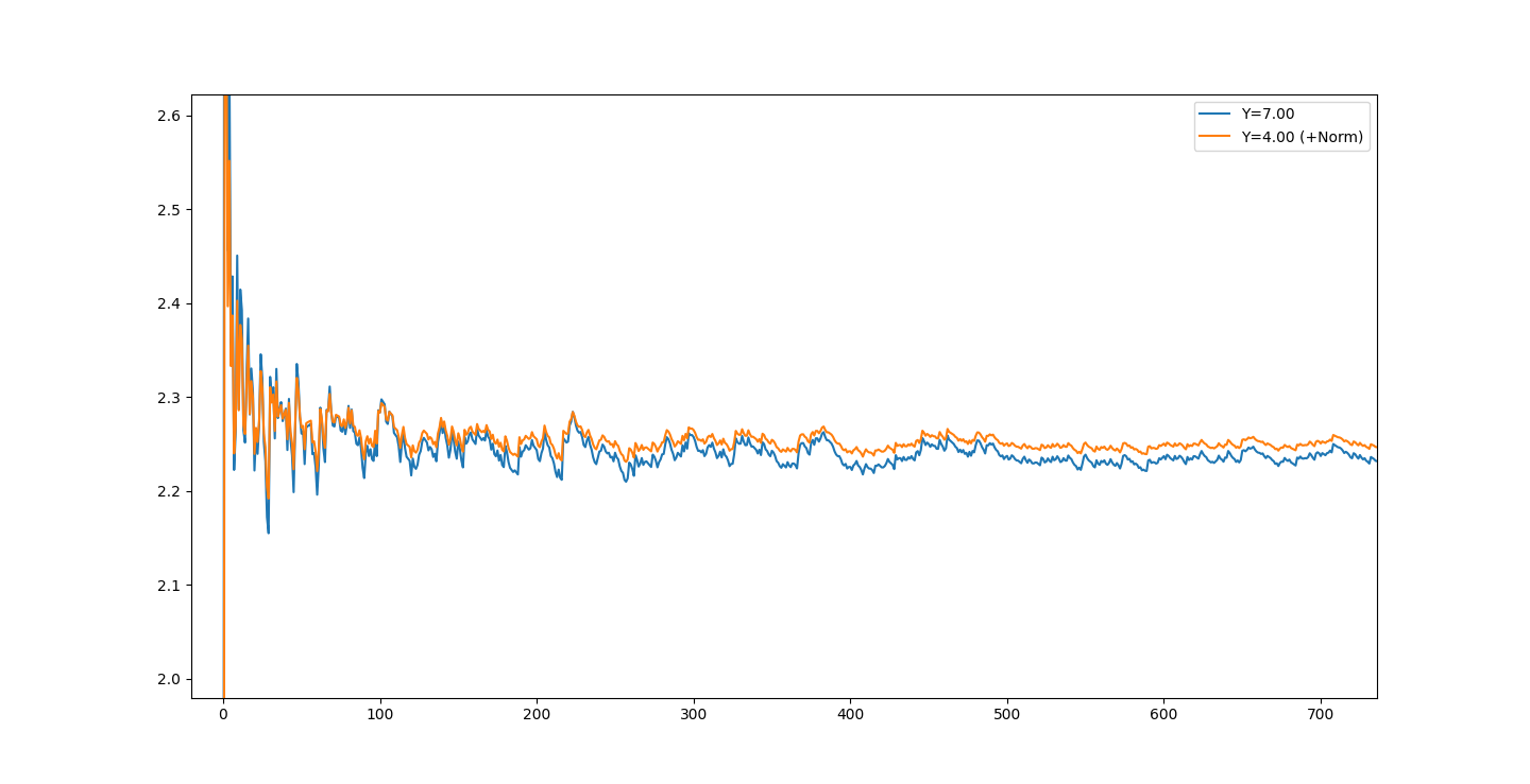
You can notice the reactivity to the values are lessened, though the plots share the same movement patterns. This is interesting - as it's dampened the amplitude to some small degree. Just changing the constant Y-value... Interesting...

Further, another smaller trivial pattern is that the mean of the A-fit values increase as we increase the Y value.

Moving back to delta distribution frequency analysis

There feels like there hasn't been as much progress using the above methods, but I still don't want to discount them. I want to move back to the idea of the distributions (pseudo-gaussian for the period of positive/negative changes in the Y-fit delta), and look at the magnitude of the change, to see if we can multiply them to get two distributions.

An idea is that if we do get two distributions (run period, as well as magnitude of values changed), we might be able to normalise the data, or run the distribution over a time period to get the Y-fit value expected to be at a certain point. We could plot magnitude by summing the change over the N period of time (a simpler distribution), or plot the values within the period, to see if there's a common sum for that number of adjustments.

Tuesday, 5th of November

I want to reflect a bit, as I feel that I have been going deeper without reflection on where we are, the goals, and the principles that may have arisen from the research.

So far, it has been a very interesting period of research on the primes. I also feel as if it's quite interesting to investigate something like the 3-body problem, but using data and future values which are known to be 100% accurate (the prime dataset). Then, to interact with this severe volatility, is rather fun.

At every depth and inspection of the differentials, we see the volatility increase in terms of deviation from the mean, and the cumulative sum of errors increases exponentially. This is fascinating - and I am sure there are other classifications of problems where these explosions in complexity exist.

Something of interest might be to contrast. To contrast the primes layers complexity rate of change (CAD), alongside the Y-fit series rate of change in complexity through deltas. If we see a lower number of complexity, maybe we're on the right track. But this is just an idea.

We started looking at groups of series, and then looked at the fitting of specific parameter values fitness. We may want to pick A, B or Y to move forward with further research, based on quantifying the volatility of values from the mean. We may also want to work out if the mean is anything of worth-ness, and if there's a trend in the mean, with something like a moving average. (I can't help myself but generate ideas as I am writing.)

Fundamentally, with the primes, I am wanting to work out a way to reduce the error at large N for the fitting of our prime curve. The way I have been doing that is fitting properties of equations I've brute-forced. If this can be done, in my opinion, we'll be able to look at the series in a new light, to see if there are other patterns that emerge when just looking at the raw complexity without the slow incremental error accumulation, and be able to layer different series onto each other to attempt to reduce the cumulative error and volatility, or solve new problems that arise.

Thursday, 7th of November

To me, this project reminds me of how success has different priorioties at different scales, and also how we tend to look at the ultra-successful for traits for their success, to think they scale to our level. This seems like an error-accumulation issue could occur, whereas we want to find an optimal "next step" for where weare. This feels related to the prime numbers we're encountering, where local properties do not marry up to the larger scale properties.

Tuesday, 12th of November

Hello!

I've been working on the ideas-side of the project, and doing a bit of experimenting. I've started a principles directory in the repo, in order to concretise some of the ideas. I've started with a period_of_change_on_fittest_values.py, to simply showcase the idea of the y-fitting, and a-fitting. This is still in progress.

As well, I've replaced the py_expression_eval with a regular function, as well as wrapped Numba around this function since it uses Numpy. This has resulted in a 10-250x speed-up depending on the system being used for computing the result of the equation, as well as a 50% increase for the Y-fitter that I've tested so far.

I am returning to the start, where we found the interesting A-fit and Y-fit pattern. As we defined above:

Y-fit has a bounded negative side.
A-fit has a bounded positive side.
The distribution of negative and positive runs are relatively known and predictable.

If there is a way to bound the negative and the positive side, then there would be no need to worry about which side of the distribution we are in (positive or negative), since we know that the positive and negative component is bounded. This is a just a theory, but I also think it adds to our aim of reducing volatility and complexity.

Working On Tweaker

I am working on an improved (DX - developer experience) tool for fitting equations. I often try to avoid using classes in engineering nowadays, but I am finding this a great use of using them to help model the complexity in the short-term. Once I complete the test, I will adjust to a functional approach if necessary. I've built it as a class which takes in a function, as well as a definition of variables. These variables can be floats (default values), they can also be LINEAR, or FITTING. Linear defines a linear series to be used (e.g. x = LINEAR, as it's 1, 2, 3, ... - this can be adjusted in the future to use other series), and FITTING indicates a value which is to be fit.

For the current "fitting" function, I am only supporting a single fitting value.

I am also getting frustrated with the complexity of the existing fitting function. It's fast, but I feel like I can remove some "fast" by restructuring it. I've asked GPT to help me, but it was useless (I didn't test too thoroughly, in honesty.) Some ideas for improving it, so it's more understandable, is to:

Use a lazy group evaluation: evaluate the step sizes we're currently on with a "shotgun" approach. Take the values for the next series of step sizes, then write an algorithm to interpret those values and decide on the direction to go.

To do this though, I might create a separate fitting function. I'll get the existing one working in the new class format, and then add in the other one. Some speed improvements may come, from being able to compute more values in bulk using Numpy and Numba.

Tweaker Update

As I finish the day, I have no important results as of yet. I have, although, been working on the tweaker, and have written a lot of code and done a lot of testing. I've tested the "shotgun" approach, and it seems to be working - but still has a lot of bloat from the refactoring I have been doing. I thought it would be simple arithmetic, though there are quite a few functions interoping in order to help solve the problem.

In this process, I had a thought: to look at the deltas of the shotgun series (shotgun: test 5 step sizes, and analyze the results). I wrote a script to test if the deltas are different with adjusted step sizes when adjusting, and they indeed are for the A-fitting. When Y-fitting - this is not the case! As we're adjusting the base logarithm. This can be factored into a separate "diff-optimisation" function, and I think the shotgun approach can be simplified a lot.

Once done, I will be able to input expressions, as well as use a flexible format in order to fit variables - so I can start to look at the relationships between A&Y fitting (finding fittings for A and Y to the primes, if that exists), as well as test more and more variants of equations. I'll keep you up to date!

November 17, 2024

Temporary hiatius. I regret to inform you that I will be doing a lot more thinking, rather than action, on this project. For the time being, I will be working over on the AI Agents research 2024 article rather than this one, though I will continue to drop in ideas from time to time which I will work through in the future.

To see the preface to the reason for this change, please read this prelude about pathways and space to see where my head is at for this reason.

I'll probably be back working on it in no time, but here are a few of the ideas I have been considering testing:

Plot the running balance of the reversals (1, 2, -4, 1 = 1, 3, -1, 0 - like betting balances) - so we can see how they trend over time. This would be better to watch the lifetime trend, instead of looking at the aggregate pseudo-gaussian values.
In the mandelbrot set, it gets more complex the closer to the center of it you get. This sounds like the ever-smaller complexity of the Y-fit values which approach some small number.
Is direction of change pseudo-gaussian, but the magnitude of change mandlebrotian? How can I identify mandlebrotian patterns, in the way I would with a gaussian?

Chat soon!